A comprehensive collection of information about real estate properties located in King County, Washington, in the United States, makes up the dataset. Each entry in the dataset, which comprises around 21600 rows and 21 columns, represents a unique property sale. The dataset contains information on a property's sale which includes its sale price, the number of bedrooms and bathrooms, the living area and lot square footage, the year the house was built, and the address of the property.

I've used a dataset which was made available on Kaggle , Here is the link for the Kaggle dataset

The initial problem at hand while analysing the dataset was to choose the method to make an appropriate model out of it. The first approach that came into thought was to use multiple linear regression because it had a lot of independent variables that could help us predict the price of the house much more accurately bu­t when multiple linear regression (MLR) is performed, it is essential to ensure that the independent variables used in the model are not highly correlated with each other. If two or more independent variables have a high correlation, it can lead to multicollinearity, which can cause issues with the model's accuracy and reliability and thus end up giving us a result which is accurate and almost close to the actual price.

the assumptions that are made while doing these analyses should also be taken into consideration

1. Linearity

2. Homoscedacity

3. Normality of Error

4. Absence of Multicollinearity

Not meeting the assumptions can lead to a poor model fit

In this study, I needed to examine the relationship between the predicted variable (price) and the independent variables (grade, bathrooms, bedrooms) to ensure that they meet the underlying assumptions.

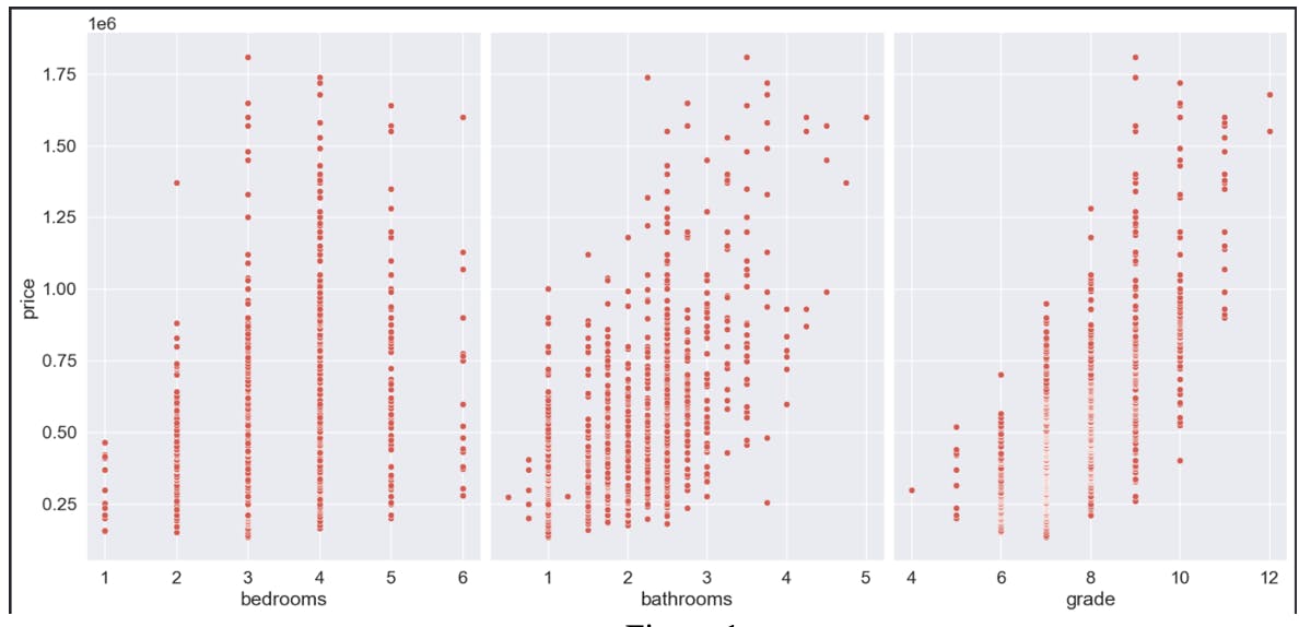
Linearity

The assumption for linearity was met for the independent variables and dependent variable as can be seen from the following graphs

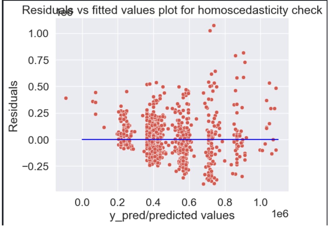
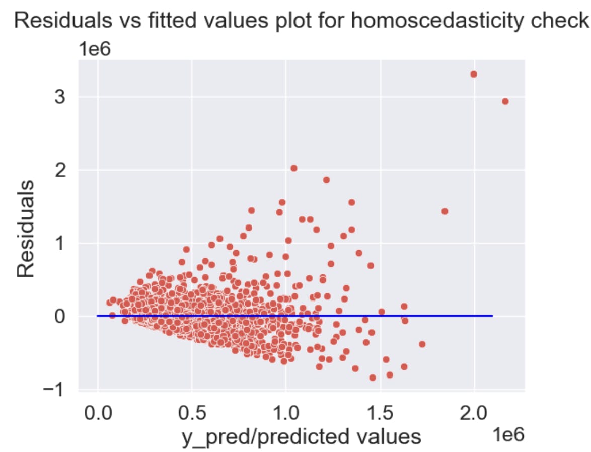
Homoscedacity

The assumption of Homoscedacity was also being met here, normally for the conditions to be met, the plot/graph must exhibit a constant spread of points across the fitted values

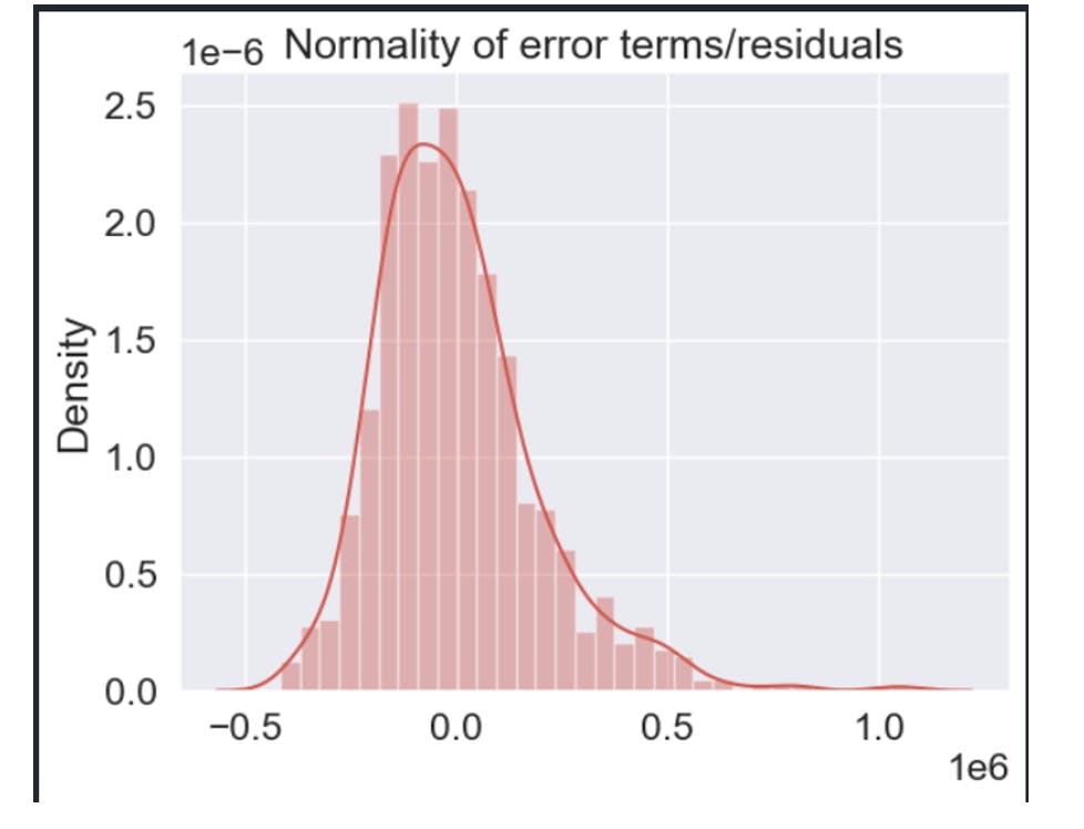
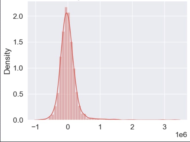
Normality

The condition for a dataset to be considered normal is that its values should follow a symmetrical and bell-shaped distribution when plotted in a graph, commonly known as the bell curve or Gaussian distribution. It can be seen in the following graph that the conditions for being normal are being met

Multicollinearity

To meet the conditions for this assumption, A correlation matrix had to be made to analyse the relation

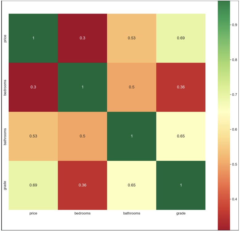
As can be seen from the matrix, grade and bathrooms had a strong correlation, so It was decided to drop the grade column or otherwise, It would have strong collinear relation between them

Model Performance

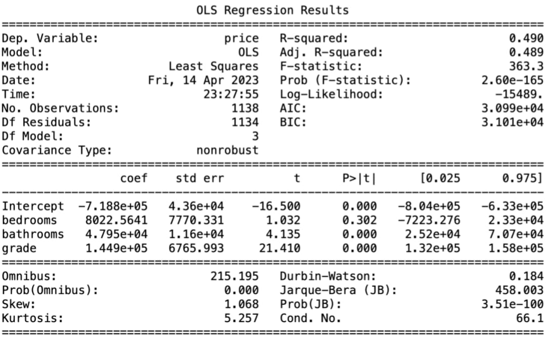
In this analysis, we have a substantial number of observations, with a total of 1,138 instances. This large sample size allows for more reliable conclusions to be drawn.

When evaluating the model's performance, I examined the F-statistic and the corresponding p-value, which was calculated to be 2.6e-165. The p-value is significantly lower than the conventional significance level of 0.05, indicating that the model performs well overall.

To assess how much of the price can be explained by the model, look at the R-squared value, which was determined to be 0.49. This means that approximately 49% of the price variation can be accounted for by the predictor variables included in the model.

To investigate the relationship between the predictor variables (bedrooms, bathrooms, and grade) and the target variable (price), I examined the coefficients, t-values, and p-values associated with each variable. The coefficients for bedrooms, bathrooms, and grades were all positive, suggesting a positive association with the price.

The p-values for bathrooms and grades were both 0, indicating that their coefficients were statistically significant, meaning they have a strong impact on the price. However, the p-value for the bedrooms coefficient was calculated to be 0.302, which is greater than the commonly used significance levels of 0.05 or 0.1. This suggests that the bedrooms variable may not be a reliable predictor of the price.

Enhancing Model Performance By Simple Linear Regression

Upon a thorough analysis of the data we can see that it is better to use a Single Linear Regression Model with sqft_living as the independent variable

The conditions for the assumptions must be met here as well

Linearity

We can see a linear relation between the dependent and independent variables, so it meets the condition here

Homoscedacity

The conditions are being met here as well as you can see the plot exhibits a constant spread of points across the fitted values except a few outliers

Linearity

As can be seen from the following graph, it follows a bell-shaped structure and thus meets the conditions

Model Performance

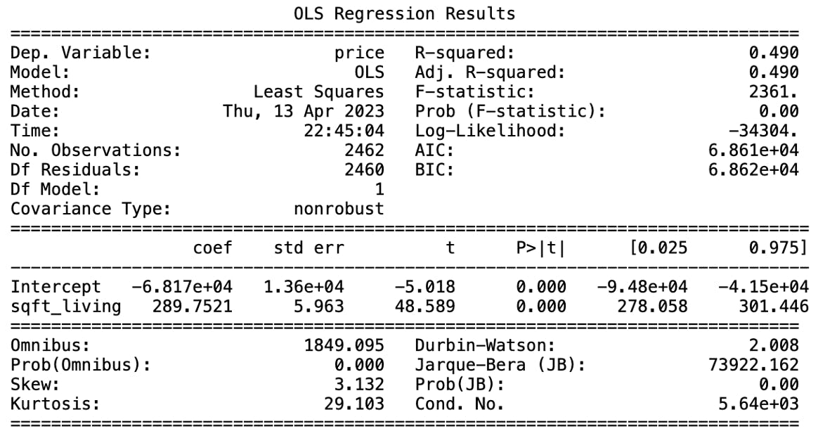
In this case, the F-statistic value of 2361 and the p-value of 0.00 tell us that the linear regression model is significant. The F-statistic is a measure of the overall fit of the model, and a high F-statistic indicates that the model fits the data well. The p-value, on the other hand, tells us the probability of obtaining a result as extreme as the one observed, assuming that the null hypothesis is true. The null hypothesis that there is no linear relationship between price and sqft_living can be rejected